🤺 Design, Analysis, and Incorporation Strategies for GeoLift Experiments

Before getting into the nitty gritty on tips on how to design, analyze, and configure experiments, it will be helpful to have a higher level overview of how GeoLift by Recast works under the hood. Like other synthetic control methodologies, GeoLift works in a fairly simple two step process:

• Construct a synthetic control such that the control and the test indicator is as close as possible before the test begins. This is demoed on the left half of the top graph with the red and blue lines.

• Estimated the incremental impact by taking the difference between the test and control after the test ends. This is illustrated with the brown area on the right side of the top graph.

The theory behind this is that if the two groups were identical in the past, any divergence must be attributable to a treatment effect. That treatment effect is the spend intervention we make on the test group.

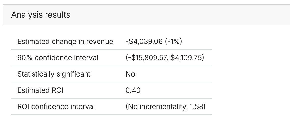
While we can report results as the estimated number of incremental conversions (or revenue) and be done, we’re usually primarily interested in the efficiency of a channel at driving conversions. To get to that, we have to know how much spend it took to cause the incremental conversions.

The second graph illustrates the change in spend during an experiment. Prior to the experiment, spend between test and control may not have been identical, but it was probably similar. We represent this area with the green shaded area above. The yellow shaded area (D) represents the drop in spend from turning off spend for the test. The purple area (B) shows a slight increase in spend in the control geographies during the test. Finally, the orange area (C) is the difference in spend expected under “business as usual” circumstances.

We can make a few observations about this graph:

• Area B + D is the amount of spend we would want to use as the “intervention” size when determining incremental CPA/ROI. This is because area C is the gap that we would expect under a business as usual situation, that would keep conversions identical to each other (like they were in the pre-test period).

• If you maintain business as usual spend perfectly in the controls, area B will be 0. This is the default recommendation on what to do that comes out of our GeoLift tool.

• Instead, if you move money from the test to the control, B will be greater than 0 (alternatively, if you move money from the control to the test, B will be negative). Note however, that moving $10,000 from test to the control will not make B and D the same size, because the red line (W) is the weighted synthetic control, not the synthetic control. You must weight the spend in each geography by it’s control weight in order to calculate W and the final size of B.

With some preliminaries out of the way, we can provide specific advice for designing and analyzing different types of tests, as well as configuring them in to your Recast MMM.

1. Test turning spend down or off

Design

Follow the basic steps in GeoLift Design, using the “decreasing spend” setting pictured below.

Analysis

Follow the basic steps in GeoLift Analyze, using the “reduced spend” setting:

What we’re really trying to provide is the size of areas B & D from the image above. If you kept spend at business as usual levels, B should be close to 0. In order to know size D, you need to construct the hypothetical line Y (the business as usual spend in the test region), and then compare the difference between Y and your actual spend. A simple way to do this would be to take an average of your recent daily spend in the test geographies, and assume business as usual spend is a continuation of this average. Then the formula for this box is just:

recent average daily spend * length of experiment - actual spend in test geopgraphies

Note that if spend is more complex, such as being highly seasonal due to recent Black Friday promotions, more complex analysis might be required.

Configuration in Recast’s MMM

If spend was turned all the way off, we’re in the simplest possible situation because the estimated ROI is equivalent to the average ROI from the first dollar spent to the business as usual spend level. In this case we can take the ROI point estimate and standard error from the results as the point estimate and uncertainty to pass to Recast (see here). The start and end dates will align to the start and end of the test (not the cooldown!), the type will be “ROI” and the Time will be “Cumulative”

If you didn’t turn spend all the way off, the result you get will not be the average ROI from $0 to the business as usual spend, but instead the average ROI from some smaller number to the business as usual spend. In this case, we can configure this as an “Impact test” to get more accurate results (note: if spend ended up quite close to 0, the differences in the two methods will be small and it is probably easier to just configure a regular ROI test). To do this we would make the following configuration changes:

• Set Type=”Impact”

• Set the point estimate to the estimated change in revenue/conversions (first row of GeoLift Analysis output)

• Set the uncertainty to (upper bound - lower bound) / 2.56 of the confidence interval on the impact (2nd row in the output)

• Set Cell1 Typical Spend Prop and Cell2 Typical Spend Prop to s1/sC where the variables are the values defined below. Cell1 and Cell2 are the same because Cell2 is the synthetic control, constructed to match Cell1.

• Set Cell1 Typical Spend Prop and Cell2 Typical Spend Prop to s1/sC where the variables are the values defined below. Cell1 and Cell2 are the same because Cell2 is the synthetic control, constructed to match Cell1.

Where

• s1 is the typical spend in the test region just before the test started

• sC is the typical spend in the entire channel just before the test started

• sT is the typical spend in the test region during the test

In general, the point estimate should be the conversions/revenue from Cell 1 minus that from Cell 2.

Note: the test does not have to be statistically significant or in the expected direction to add to the MMM. In fact, if you only include statistically significant experiments, you risk biasing your model to too high ROIs by omitting the small effects.

2. Test turning spend up

Design

Follow the basic steps in GeoLift Design, using the “increasing spend” setting pictured below.

Analysis

Follow the basic steps in GeoLift Analyze, using the “increased spend” setting

What we’re really trying to provide is the size of areas B & D from the image above, except in this case Z should be higher than W, so things will be flipped. If you kept spend at business as usual levels, B should be close to 0. In order to know size D, you need to construct the hypothetical line Y (the business as usual spend in the test region), and then compare the difference between your actual spend and Y. A simple way to do this would be to take an average of your recent daily spend in the test geographies, and assume business as usual spend is a continuation of this average. Then the formula for this box is just:

Actual spend in test geographies - Recent average daily spend * Length of experiment

If spend is more complex, such as being highly seasonal due to recent Black Friday promotions, more complex analysis might be required.

Configuration in Recast MMM

Because we are not measuring the ROI from going from $0 of spend to another level of spend, we want to configure this as an “Impact test” to get the most accurate results (note: if business as usual spend is quite close to $0, this can be configured as a as a regular ROI test). To do this we would make the following configuration changes:

• Set Type=”Impact”

• Set the point estimate to the estimated change in revenue/conversions (first row of GeoLift Analysis output)

• Set the uncertainty to (upper bound - lower bound) / 2.56 of the confidence interval on the impact (2nd row in the output)

• Set Cell1 Typical Spend Prop and Cell2 Typical Spend Prop to s1/sC where the variables are the values defined below. Cell1 and Cell2 are the same because Cell2 is the synthetic control, constructed to match Cell1.

• Set Cell1 Typical Spend Prop and Cell2 Typical Spend Prop to s1/sC where the variables are the values defined below. Cell1 and Cell2 are the same because Cell2 is the synthetic control, constructed to match Cell1.

Where

• s1 is the typical spend in the test region just before the test started

• sC is the typical spend in the entire channel just before the test started

• sT is the typical spend in the test region during the test

In general, the point estimate should be the conversions/revenue from Cell 1 minus that from Cell 2.

Note: the test does not have to be statistically significant or in the expected direction to add to the MMM. In fact, if you only include statistically significant experiments, you risk biasing your model to too high ROIs by omitting the small effects.

3. Test spend down; control spend up

Design

You can design a test as you normally would (see here), but interpret the results slightly differently. Instead of taking the recommendation to spend $x less in the test geographies, you can interpret it as the difference in spend you need to achieve between the test group and the synthetic control. You basically get to double count the proportion of spend that moves from the test group into the synthetic control. The amount that moves into the synthetic control is proportional to the size of the test group, so we first need to figure out the size of the synthetic control, which is constructed to be the size of the test group.

We can calculate the size of the test group by taking the proportion of the dependent variable (revenue/conversions) that typically happens in the test group relative to the total. Let’s call this p.

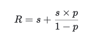
If we reduce spend in the test group and spread it out evenly across all control geographies, the amount that moves into the synthetic control is spend*p/(1-p) because 1-p is the size of the control as a whole and p is the size of the synthetic control, so p/(1-p) is the proportion of spend that you get to “double count” because it moved into the synthetic control. If p=0.5, so that the test is an exact split of your geographies, we see that 100% of the spend is double counted because all control geographies are part of the synthetic control.

So for a GeoLift recommendation of R dollars, we can calculate how much we should actually reduce spend using this formula:

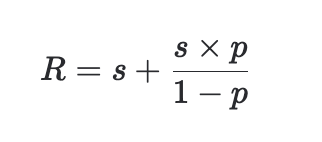
s is the spend held out of the test, s*p/(1-p) is the amount of spend we get to double count because it moves into the synthetic control. Solving for s we get:

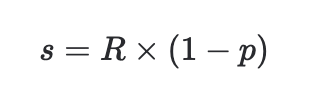
which is the total amount of spend we should move from the test to the control. For example, if GeoLift recommends cutting spend by 30,000, and our test regions make up 15% of our business, we can instead move $25,500 (30k/(1+0.15/0.85)) out of the test region, spread it through the control regions, and get the same effect.

Analysis

If you followed the steps laid out in the Design stage, the analysis should be straightforward (see here). You should be able to use the spend recommendation from the design as the dollar amount if you followed the plan. If the plan didn’t go quite as expected. For example, you weren’t able to make the cuts as deeply as you wanted or you weren’t able to reallocate all the money to the controls, you may need to adjust this number up or down to reflect what actually happened.

Configuration in Recast MMM

See Section 5: “Configuration for any two-celled test”

4. Test spend up; control spend down

Design

You can design a test as you normally would (see here), but interpret the results slightly differently. Instead of taking the recommendation to spend $x more in the test geographies, you can interpret it as the difference in spend you need to achieve between the test group and the synthetic control. You basically get to double count the proportion of spend that moves to the test group from the synthetic control. The amount that moves from the synthetic control is proportional to the size of the test group, so we first need to figure out the size of the synthetic control, which is constructed to be the size of the test group.

We can calculate the size of the test group by taking the proportion of the dependent variable (revenue/conversions) that typically happens in the test group relative to the total. Let’s call this p.

If we increase spend in the test group and remove it evenly across all control geographies, the amount that moves out of the synthetic control is spend*p/(1-p) because 1-p is the size of the control as a whole and p is the size of the synthetic control, so p/(1-p) is the proportion of spend that you get to “double count” because it moved out of the synthetic control into the test. If p=0.5, so that the test is an exact split of your geographies, we see that 100% of the spend is double counted because all control geographies are part of the synthetic control.

So for a GeoLift recommendation of R dollars, we can calculate how much we should actually increase spend using this formula:

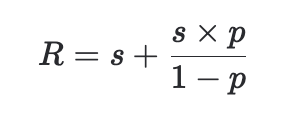
s is the spend moved to the test, s*p/(1-p) is the amount of spend we get to double count because it moves out of the synthetic control. Solving for s we get:

which is the total amount of spend we should move from the control regios to the test. For example, if GeoLift recommends increasing spend by 30,000, and our test regions make up 15% of our business, we can instead increase $25,500 (30k/(1+0.15/0.85)) in the test region, taking it from the controls, and get the same effect.

Analysis

If you followed the steps laid out in the Design stage, the analysis should be straightforward (see here). You should be able to use the spend recommendation from the design as the dollar amount if you followed the plan. If the plan didn’t go quite as expected. For example, you weren’t able to increase the spend as much as you wanted, you may need to adjust this number up or down to reflect what actually happened.

Configuration in Recast MMM

See Section 5: “Configuration for any two-celled test”

5. Configuration for any two-cell-test

You can use this configuration for any two-cell test:

• Set Type=”Impact”

• Set the point estimate to the conversions/revenue in Cell 1 minus that from Cell 2

• Set the uncertainty to the standard error of the above difference. If you have an 80% confidence interval for that difference, then set the uncertainty to (upper bound - lower bound) / 2.56 of the confidence interval.

• Set Cell1 Typical Spend Prop to s1/sC and Cell2 Typical Spend Prop to s2/sC where the variables are defined below.

• Set Cell1 Test Spend Ratio to s1T/s1 and Cell2 Test Spend Ratio to s2T/s2 where the variables are defined below

Where:

• s1 is the typical spend in Cell 1 just before the test started

• s2 is the typical spend in Cell 2 just before the test started

• sC is the typical spend in the entire channel just before the test started

• s1T is the typical spend in Cell 1 during the test

• s2T is the typical spend in Cell 2 during the test

In general, the point estimate should be the conversions/revenue from Cell 1 minus that from Cell 2.

Note: the test does not have to be statistically significant or in the expected direction to add to the MMM. In fact, if you only include statistically significant experiments, you risk biasing your model to too high ROIs by omitting the small effects.